Understand and Apply Stereo Rectification for Depth Maps (Part 2)

In part 1 of the article series, we’ve identified the key steps to create a depth map. We have captured a scene from two distinct positions and loaded them with Python and OpenCV. However, the images don’t line up perfectly fine. A process called stereo rectification is crucial to easily compare pixels in both images to triangulate the scene’s depth!

For triangulation, we need to match each pixel from one image with the same pixel in another image. When the camera rotates or moves forward / backward, the pixels don’t just move left or right; they could also be found further up or down in the image. That makes matching difficult.

Wrapping Images for Stereo Rectification

Image rectification wraps both images. The result is that they appear as if they have been taken only with a horizontal displacement. This simplifies calculating the disparities of each pixel!

With smartphone-based AR like in ARCore, the user can freely move the camera in the real world. The depth map algorithm only has the freedom to choose two distinct keyframes from the live camera stream. As such, the stereo rectification needs to be very intelligent in matching & wrapping the images!

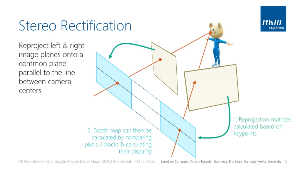
In more technical terms, this means that after stereo rectification, all epipolar lines are parallel to the horizontal axis of the image.

To perform stereo rectification, we need to perform two important tasks:

Detect keypoints in each image.
We then need the best keypoints where we are sure they are matched in both images to calculate reprojection matrices.
Using these, we can rectify the images to a common image plane. Matching keypoints are on the same horizontal epipolar line in both images. This enables efficient pixel / block comparison to calculate the disparity map (= how much offset the same block has between both images) for all regions of the image (not just the keypoints!).

Google’s research improves upon the research performed by Pollefeys et al. . Google additionally addresses issues that might happen, especially in mobile scenarios.

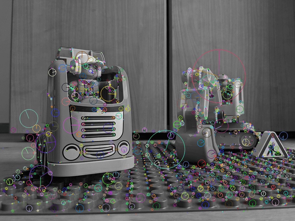
2a) Detecting Keypoints

But how does the complete stereo rectification process work? Let’s build our own code to better understand what’s happening. In the ideal case, you’d have a calibrated camera to start with. But it also works satisfactory without prior calibration.

The code is not exactly what Google built. But it’s using well-known and established open-source algorithms instead.

OpenCV has a tutorial that lists multiple ways of matching features between frames. In the Simultaneous Localization and Mapping (SLAM) article series, I provided some background on different algorithms and showed how they work. Here, we’ll use the traditional SIFT algorithm. Its patent expired in March 2020, and the algorithm got included in the main OpenCV implementation.

To get a feeling for the image, this is what the keypoints look like from the left image (img1):

2b) Matching Keypoints

The code calculated keypoints individually for each image. As these are taken from a slightly different perspective, there will also be differences in the detected points. As such, to perform stereo rectification, we next need to match the keypoints between both images. This allows to detect which are present in both images, as well as their difference in the position.

An efficient algorithm is the FLANN matcher. It sorts the best potential matches between similar keypoints in both frames based on their distance using a K-nearest-neighbor search.

However, this usually provides far more matches than we need for the following steps. Therefore, the next few lines of code go through the keypoint matches and select the best ones, as described by Lowe .

To visually check the matches, we can also draw these. As there are still a lot of matches left, I’m just selecting a few of the matches [300:500]. If your source images have fewer matches, remove the array selection to draw all of them!

2c) Stereo Rectification

The matching we have performed so far is a pure 2D keypoint matching. However, to put the images in a 3D relationship, we should use epipolar geometry. A major step to get there: the fundamental matrix describes the relationship between two images in the same scene. It can be used to map points of one image to lines in another.

What exactly is Epipolar Geometry? The “Computer Vision” course of the Carnegie Mellon University has excellent slides that explain the principles and the mathematics. This part of their course is also using the Computer Vision: Algorithms and Applications book as source. Its second edition is currently in the works and can be read for free online at the author’s website. Here, I’ll just explain the basics without the mathematical background.

In the following example, we observe a cat looking at a mouse. While the cat sees various keypoints of the mouse as points in her field of vision, we “see” the lines between the cat’s eyes and the mouse’s features as lines.

The origin of the lines we observe is the epipole, and the lines are the epipolar lines.

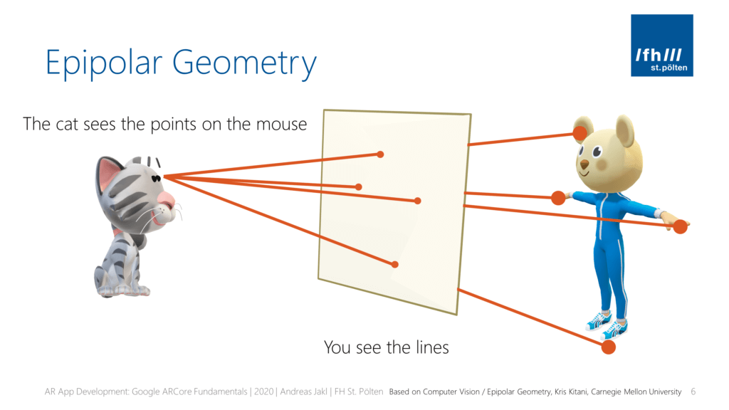
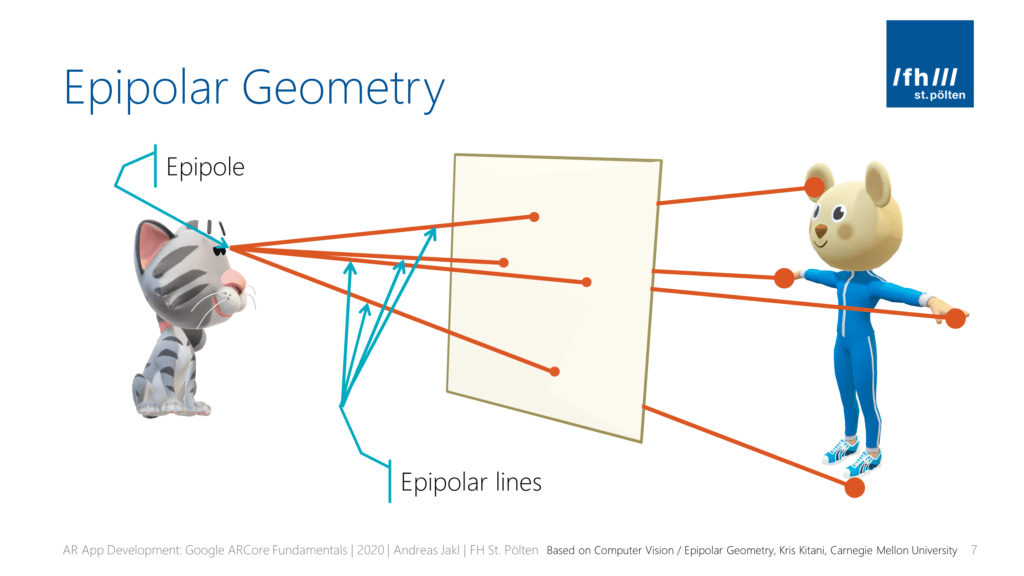
Of course, this example directly transfers to the cat being one camera o, and we as observers being the other camera o'. Both cameras see the same keypoint of the scene p (the mouse). In a more formalized way, we can represent the same setup in the following image.

Epipolar Constraint

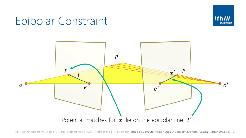
The rectangles shown in perspective are the image planes of both cameras. The same keypoint p is visible at different positions x and x' in both images. However, they won’t be at the same position:

Remember that in the end, we need a disparity between both images to estimate the depth: objects that are closer to the (horizontally) moving camera will have a greater offset when comparing two keyframes, while objects that are far away will be at roughly the same position in both images.

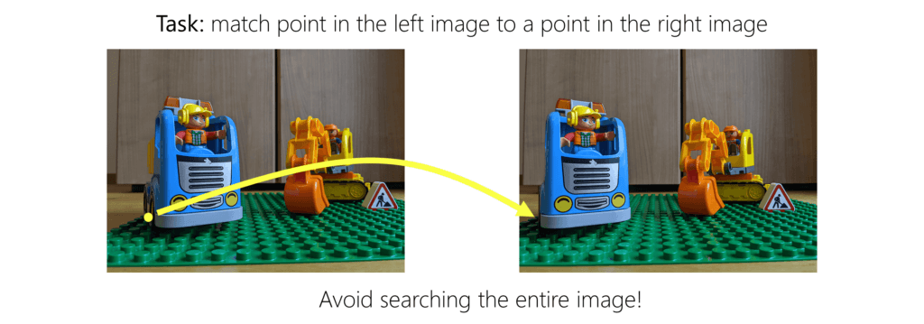
So, how do we find the match x' in the second image? Keep in mind that we shouldn’t just find matches for the keypoints, but for each pixel / block in the whole image to make the disparity map as dense as possible!

Luckily, when we know the reprojection matrix between both images, the epipolar constraint tells us that the matching pixel / block x' in the image o' is on the epipolar line l'. Otherwise, we’d have to search the whole image to find a good match.

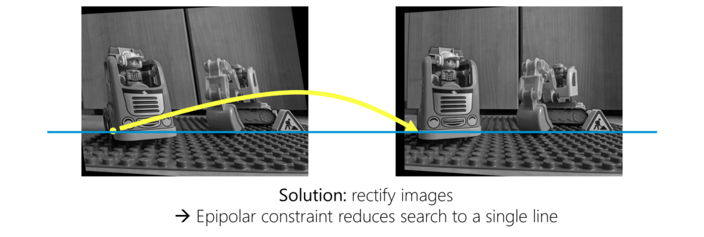
Epipolar Lines for Stereo Rectification

These epipolar lines (epilines) will be at an angle in both images. That makes matching more computationally difficult. Stereo rectification reprojects the images to a new common plane parallel to the line between the camera centers.

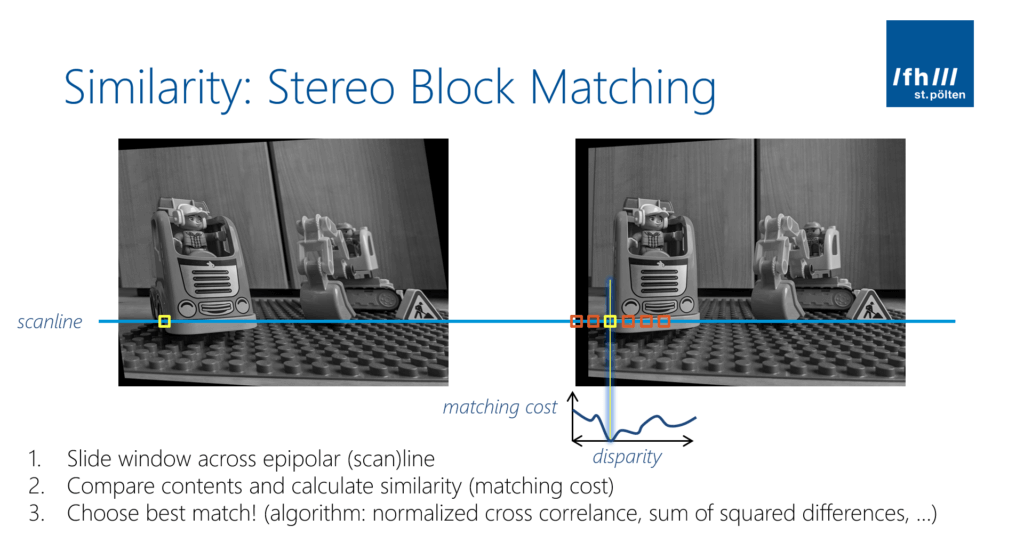
So, if the images are rectified, this means that calculating the disparity is a simple search along the corresponding horizontal epipolar line in the other image.

Why is the matching so simple now that we have rectified the images? We only need to use a simple block comparison algorithm. It compares a block in the left image with blocks in the right image at different disparities. The winner is the block with the minimum matching cost. The algorithm is usually a normalized cross correlation (NCC) or the sum of absolute differences (SAD). Speed matters, as we perform this operation for every block in the image to generate a full disparity map!

Fundamental Matrix

How do we rectify images in code? The essential matrix allows us to calculate the epipolar line in the second image given a point in the first image. The fundamental matrix is a more generalized version of the same concept. Given that, we can also rectify the images (= undistort), so that the images are wrapped in a way that their epilines are aligned.

OpenCV includes a function that calculates the fundamental matrix based on the matched keypoint pairs. It needs at least 7 pairs but works best with 8 or more. We have more than enough matches. This is where the RanSaC method (Random Sample Consensus) works well. RANSAC also considers that not all matched features are reliable. It takes a random set of point correspondences, uses these to compute the fundamental matrix and then checks how well it performs. When doing this for different random sets (usually, 8-12), the algorithm chooses its best estimate. According to OpenCV’s source code, you should have at least fifteen feature pairs to give the algorithm enough data.

The tutorial by OpenCV about epipolar geometry has more background info about the process. Here the adapted source code that fits to our application:

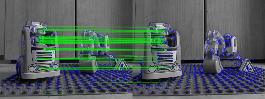
Epilines

This is enough to find epilines. You can see their visualization in the image below. The Python code marked corresponding keypoints in both images. As you can observe, they lie on the same epipolar lines.

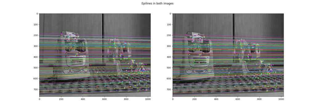
In this case, there is not much difference between the images, as they are taken with a small baseline distance from roughly the same angle. In case the camera angle would be more drastically different as seen in the OpenCV tutorial, you’d note that the lines diverge more.

The code to create this visualization is slightly improved from the tutorial. I’ve initialized the random number generator so that the colors of the lines in both images match, making the images easier to compare.

Source Code for Stereo Rectification

How do we get the stereo rectified images? After all the preparatory steps, performing the actual stereo rectification through OpenCV is remarkably short and easy.

As we did not perform a specific camera calibration, we will use the uncalibrated version of the algorithm. Of course, this introduces further inaccuracies to an already sensitive system, given all the potential small errors that can accumulate. But in many cases, it still provides satisfactory results.

To perform the rectification, we simply pass the matched points from both images as well as the fundamental matrix into the stereoRectifyUncalibrated() method. OpenCV’s implementation is based on Hartley et al. .

What we get back are the planar perspective transformations encoded by the homography matrices H1 and H2. A homography matrix maps a point to a point, while the essential matrix maps a point to a line.

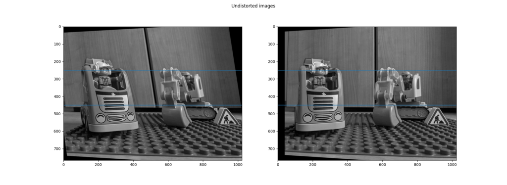
Now let’s see if this improved the image alignment. Using OpenCV’s warpPerspective() function, we can apply the calculated transformations to the source images.

As you can see, both source images have now changed. The same two blue horizontal lines are drawn on top of the images. Look closely at the distinct features in both images and compare them: they lie exactly on the same line in their respective image. A good reference point is the eye of the construction worker figure in the car.

Article Series

Now our images are prepared. Read the next part to see how to perform matching to generate the disparity maps!