How to Apply Stereo Matching to Generate Depth Maps (Part 3)

In part 2, we rectified our two camera images. The last major step is stereo matching. The algorithm that Google is using for ARCore is an optimized hybrid of two previous publications: PatchMatch Stereo and HashMatch .

An implementation in OpenCV is based on Semi-Global Matching (SGM) as published by Hirschmüller . In Google’s paper , they compare themselves to an implementation of Hirschmüller and outperform those; but for the first experiments, OpenCV’s default is good enough and provides plenty of room for experimentation.

3. Stereo Matching for the Disparity Map (Depth Map)

OpenCV documentation includes two examples that include the stereo matching / disparity map generation: stereo image matching and depth map.

Most of the following code in this article is just an explanation of the configuration options based on the documentation. Setting fitting values for the scenes you expect is crucial to the success of this algorithm. Some insights are listed in the Choosing Good Stereo Parameters article. These are the most important settings to consider:

• Block size: if set to 1, the algorithm matches on the pixel level. Especially for higher resolution images, bigger block sizes often lead to a cleaner result.
• Minimum / maximum disparity: this should match the expected movements of objects within the images. In freely moving camera settings, a negative disparity could occur as well – when the camera doesn’t only move but also rotate, some parts of the image might move from left to right between keyframes, while other parts move from right to left.
• Speckle: the algorithm already includes some smoothing by avoiding small speckles of different depths than their surroundings.

Visualizing Results of Stereo Matching

I’ve chosen values that work well for the sample images I have captured. After configuring these values, computing the disparity map is a simple function call supplying both rectified images.

The last few lines of code just normalize the resulting values to a range of 0..255 so that they can be directly shown and saved as a grayscale image. This is what the result looks like:

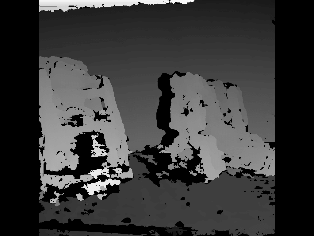
As you can see, the depth map looks good! It’s easy to recognize the car and the different depths of the excavator.

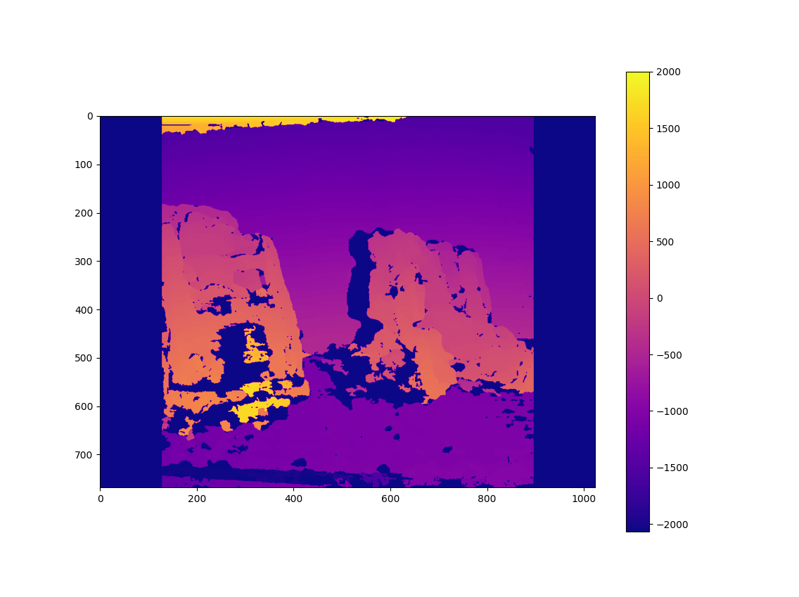
If you prefer a more colorful disparity map, you can also draw the image using a colormap; in this case, I’ve chosen a perceptually uniform sequential colormap. I’ve fed in the non-normalized disparity map.

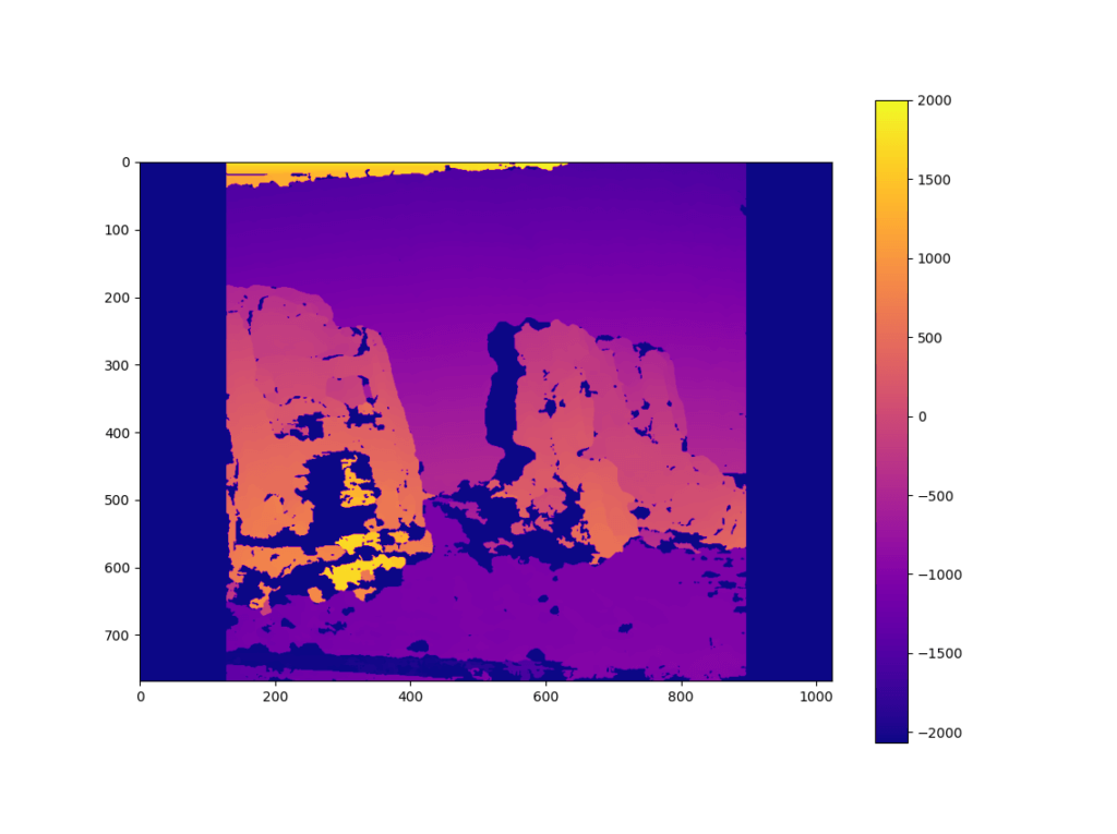
The background looks surprisingly well too, given that it is an almost untextured surface. If you look at the SIFT features that we calculated previously in this article series, it didn’t find many keypoints in that area.

On the other hand, the floor was a bit more problematic for the depth map, which is in part also related to its repeating texture that is problematic for purely optical matching algorithms. Further tweaking of the disparity map generation settings could improve the results here as well.

Next Steps: Filtering & Point Cloud

The depth map we generated is sparse. This means that it only contains information in textured regions; you can clearly see that it struggled calculating the depth in the excavator’s shovel.

This is a good example of a region with insufficient texture. Another issue are regions that are only visible in one of the images but occluded in the other. As such, to generate a full depth map, you should also apply filtering to fill these gaps. An example can be found in the OpenCV Disparity map post-filtering article.

Additionally, our depth map process would be temporally inconsistent and is not aligned to edges of the image. Google optimized the depth maps in ARCore using bilateral solver extensions . However, we won’t go into details here.

Another task would be creating a point cloud based on the disparity map. OpenCV stereo_match.py sample shows some sample code for this.

Also note that our disparity map doesn’t directly reveal the distance in meters, so you’d have to convert the values of the disparity map to depth. Depending on the exact system setup (polar rectification vs. other methods), this can be trivial or a more complex triangulation.

Article Series

We finished exploring the background of generating depth maps. How to apply that to AR Foundation, and how does the official depth map sample app compare? Read the next part!

1. Easily Create Depth Maps with Smartphone AR (Part 1)
2. Understand and Apply Stereo Rectification for Depth Maps (Part 2)
3. How to Apply Stereo Matching to Generate Depth Maps (Part 3)
4. Compare AR Foundation Depth Maps (Part 4)
5. Visualize AR Depth Maps in Unity (Part 5)

Bibliography