Creating apps that work well with Augmented Reality requires some background knowledge of the image processing algorithms that work behind the scenes. One of the most fundamental concepts involves anchors. These rely on keypoints and their descriptors, detected in the recording of the real world.
Anchor Virtual Objects to the Real World
AR development APIs hide much of the complexity. As a developer, you simply anchor virtual objects to the world. This ensures that the hologram stays glued to the physical location where you put it.
Objects stay in place even if the system learns more about the environment over time. For example, you place an object on the wall 2 meters away from you. Next, you walk closer to the wall. The sensors got more accurate measurements of the distances and find out that the wall would’ve actually been 2.1 meters away from your original position, instead of just 2.0 meters. The engine needs to reflect this new knowledge in the 3D object position.
In a traditional single world-coordinate system, every object has fixed x, y, z coordinates. Anchors override the position and rotation of the transform component attached to the 3D object. The perceived real world has priority over the static coordinate system.
How are Anchors “Anchored”?
But how do the anchors make objects stick to real-world positions?
The Google ARCore documentation reveals that anchors are based on a type called “trackables” – detected feature points and planes. As planes are grouped feature points which share the same planar surface, it all comes down to feature points.
The following video shows feature points detected by Google ARCore. They’re marked as turquoise dots. As you can see, ARCore detects a large number in the concrete pillar. It has a very visible texture. However, not a single feature point is found in the white walls. Also, the wooden windowsill is very smooth and tricky to detect.
Feature Points in Computer Vision
What is a feature point? It’s a distinctive location in images – for example corners, blobs or T-junctions are usually good candidates. This information alone wouldn’t be enough to distinguish one from another, or to reliably find feature points again. Therefore, also the neighborhood is analyzed and saved as a descriptor.
The most important property of a good feature point is reliability. The algorithm must be able to find the same physical interest point under different viewing conditions. A lot can change while you’re using an AR app:
- camera angle / perspective
- rotation
- scale
- lightning
- blur from motion or focusing
- general image noise
Finding Reliable Feature Points
How do the AR frameworks find features? The Microsoft HoloLens operates with an extensive amount of sensor data. Especially the depth information based on reflected structured infrared light is valuable. Mobile AR like Google ARCore and Apple ARKit can only work with a 2D color camera.
Finding distinctive feature points in images has been an active research field for quite some time. One of the most influential algorithms is called “SIFT” (“Scale Invariant Feature Transform”). It was developed by David G. Lowe and published in 2004. Another “traditional” method is called “SURF” (Speeded up robust features”) by H. Bay et al. Both are still in use today. However, both algorithms are patented and usually too slow for real-time use on mobile devices.
It’s not publicly known which algorithms are used by the Windows Mixed Reality, ARCore and ARKit. However, several robust and patent-free algorithms exist.
A good candidate is the “BRISK” (“Binary Robust Invariant Scalable Keypoints”) algorithm by Leutenegger et al. It’s fast and efficient enough to serve as base of the overall “SLAM” approach of simultaneously locating the camera position and mapping the real world.
How is a Feature Detected and Stored? With Keypoints!
Feature detection is a multi-step process. Its components vary depending on the algorithms. A short description of a typical detection algorithm:
1. Keypoint Detection
This can for example be a corner-detection algorithm that considers the contrast between neighboring pixels in an image.
To make the feature point candidates scale-invariant and less dependent on noise, it’s common to blur the image. Differently scaled variants of the image (octaves) improve scale independence. A good explanation is that you’d typically want to detect a tree as a whole to achieve reliable tracking; not every single twig. The SIFT and SURF algorithms use this approach.
Unfortunately, blurring is computationally expensive. For real-time scenarios, other algorithms like BRISK can provide a better overall experience. These algorithms (including BRISK) are often based on a derivative of the FAST algorithm by Rosten and Drummond.
FAST analyzes the circular surroundings of each pixel p. Is the surrounding pixel’s brightness lower / higher than of p (including a threshold)? If a certain number of connected pixels fulfill this criterion, the algorithm has found a corner. This is indicated by the dotted line in the image below. Pixels 7 to 10 are darker than p; the others are brighter.
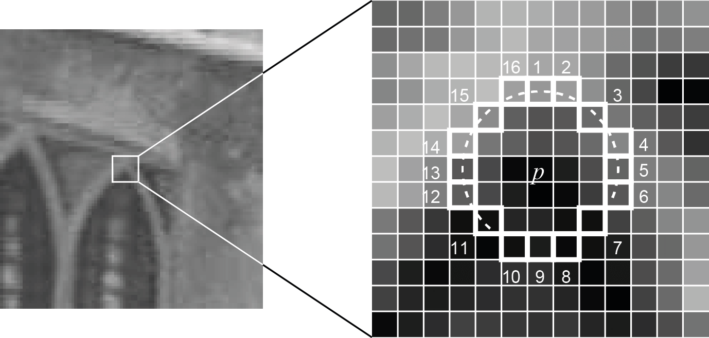
For BRISK, at least 9 consecutive pixels in the 16-pixel circle must be sufficiently brighter or darker than the central pixel. In addition, BRISK also uses down-sized images (scale-space pyramid) to achieve better invariance to scale – even reaching sub-pixel accuracy.
2. Keypoint Description
Each of all the detected keypoints need to be a unique fingerprint. The algorithm must find the feature again in a different image. This might have a different perspective, lightning situation, etc. Even under these circumstances, a match has to be possible.
The BRISK descriptor is a binary string with 512 bits. Essentially, it’s a concatenation of brightness comparison results between different samples surrounding the center keypoint.
As shown in the figure, the blue dots form the concentric circles for the sampling positions. The red circles indicate the individually sampled areas, based on a Gaussian smoothing to avoid aliasing effects.
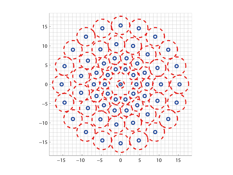
Based on these sampling points, the results of brightness comparisons are calculated – depending on which sample is brighter, it results in 0 or 1.
Additionally, BRISK ensures rotational invariance by calculating the characteristic direction. This is determined by the largest gradients between two samples with a long distance from each other. Essentially, this means: at which angle would a cut through the keypoint area result in the biggest brightness difference between either side of the cut?
The Code: Testing BRISK with OpenCV and Python
It’s time to test the algorithm in practice. The OpenCV library is one of the most commonly used frameworks for image processing. It contains reference implementations for many different feature detection algorithms. These include the BRISK algorithm. SIFT and SURF have been moved to a separate extra module, as they are patented.
To get started, install the latest version of Python 3.x+ and Visual Studio Code. Then, download the official Python extension from Microsoft. The documentation contains a full tutorial of the integration between Visual Studio Code and Python.
OpenCV 3 and Python 3
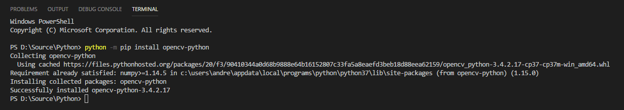
Thankfully, the community already provides a pre-compiled OpenCV package with complete Python bindings. Using the pip package manager, you can install the opencv-python module with the following command from PowerShell or from the terminal within Visual Studio Code:
python -m pip install opencv-python
If you’d like to try SIFT and SURF as well, additionally get the opencv-contrib-python module. Also see the article from Michael Hirsch for reference.
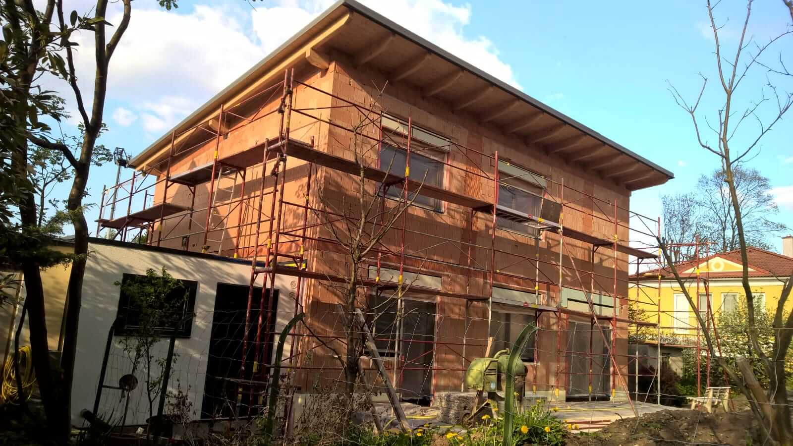
As test image for the feature detection, I’m using a photo of my construction site. The photo has areas with little contrast in the sky, as well as lots of corner element in various contrasts – ranging from artificial corners in scaffolding to trees.
Visualizing Feature Points
I’ve written a small script to test where features are detected.
import cv2       # OpenCV

# 1. Load the original image
img = cv2.imread('house.jpg')
# Convert the image to grayscale
gray = cv2.cvtColor(img, cv2.COLOR_BGR2GRAY)

# 2. Create BRISK algorithm
# OpenCV default threshold = 30, octaves = 3
# Using 4 octaves as cited as typical value by the original paper by Leutenegger et al.
# Using 70 as detection threshold similar to real-world example of this paper
brisk = cv2.BRISK_create(70, 4)

# 3. Combined call to let the BRISK implementation detect keypoints
# as well as calculate the descriptors, based on the grayscale image.
# These are returned in two arrays.
(kps, descs) = brisk.detectAndCompute(gray, None)

# 4. Print the number of keypoints and descriptors found
print("# keypoints: {}, descriptors: {}".format(len(kps), descs.shape))
# To verify: how many bits are contained in a feature descriptor?
# Should be 64 * 8 = 512 bits according to the algorithm paper.
print(len(descs[1]) * 8)

# 5. Use the generic drawKeypoints method from OpenCV to draw the
# calculated keypoints into the original image.
# The flag for rich keypoints also draws circles to indicate
# direction and scale of the keypoints.
imgBrisk = cv2.drawKeypoints(gray, kps, img, flags=cv2.DRAW_MATCHES_FLAGS_DRAW_RICH_KEYPOINTS)

# 6. Finally, write the resulting image to the disk
cv2.imwrite('brisk_keypoints.jpg', imgBrisk)
After importing the OpenCV module, the code performs the following steps:
- Image loading: Loads the original JPEG image (into variable img ) and converts it to gray-scale ( gray ), as this is the base for the algorithm. If you’re working with a live camera that provides other color streams than RGB, you could skip the conversion step and for example work directly with the Y channel from YUV.
- BRISK algorithm: In this step, the BRISK algorithm gets initialized. OpenCV contains a configurable reference implementation of the algorithm. In my case, I’ve used 4 octaves instead of the default 3 (the number of image scale series used). Additionally, I’ve increased the threshold to get less but more reliable keypoints.
- Keypoints & Descriptors: you could split keypoint detection and keypoint description into two separate steps. This would allow you to use different algorithms for each step. As BRISK contains implementations for both parts, you can use the combined method detectAndCompute() . It returns two arrays: the detected keypoints, as well as their respective descriptors.
- Verify: this step is just to print how many keypoints have been detected. Also, as explained above, the BRISK algorithm provides feature vectors with 512 binary numbers.
- Visualize: this step is a generic method of OpenCV to draw keypoints at their detected positions into an image, for debugging & verification. I used the optional flag DRAW_MATCHES_FLAGS_DRAW_RICH_KEYPOINTS. Instead of simply drawing a dot at each keypoint location, the method now additionally indicates the keypoint size and orientation through the circle diameter and the angle.
- Save: the last step simply stores the image with the visualized keypoints to a JPG file:
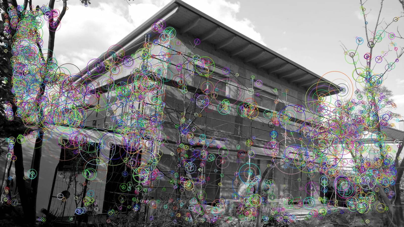
As expected, most keypoints are visible in areas with distinct edges. This includes the scaffolding, windows, doors and trees. The sky doesn’t contain a single keypoint. Due to the high threshold, there are also no keypoints in the ceiling, as the contrast is rather low in these areas.
Summary of Feature Detection
With this article, we looked at one of the most important background technologies that enable Augmented Reality with spatial anchors. Design your apps so that users place objects in areas where the device has a chance of creating anchors.
An example: placing lots of virtual pictures on a wall usually leads to a bad AR experience – it’s just too difficult to detect keypoints on plain surfaces. As a result, tracking of the anchored real-world position easily gets inaccurate and the hologram doesn’t stay in place.
If your game or app design mainly focuses on placing objects closer to corners of the floor or the table, the app will work much better. This design ensures that the algorithms will always find enough keypoints close to the anchor.
Additionally, read the recommendations from Microsoft and Google regarding the use of spatial anchors. Most important:
- Release spatial anchors if you don’t need them. Each spatial anchor costs CPU time, as the AR framework prioritizes these areas to get a stable tracking around the anchors.
- Keep the object close to the anchor. Don’t use the transformation matrix of the (child)objects to move the object too far from the anchor. Microsoft recommends a maximum of 3 meters. Considering the less accurate tracking on camera-only systems like ARCore and ARKit, I’d recommend a lot less distance for phone-based AR.
Additional pointers: OpenCV & Unity
To integrate OpenCV with Unity for use in HoloLens, ARCore and ARKit projects, you can handle the integration manually. The Unity forms contain a good and helpful discussion of the required steps. Of course, you can also choose the easy route and purchase the OpenCV for Unity asset from the Unity store.